
This post is part of a series in which I’m discussing several parts of my AI_at_Rappi presentation. In the last two posts, we first discussed how to evaluate a churn marketing campaign using a financial evaluation measure and then how to estimate the customer lifetime value and also how it is possible to design experiments to estimate the probability of an offer acceptance gamma. Finally, in this last part, we want to discuss how to include cost-sensitive machine learning algorithms into this analysis.
First, we need to understand what is the difference between classical machine learning algorithms and cost-sensitive classification.
Cost-sensitive Machine Learning
Classification in the context of machine learning, deals with the problem of predicting the class 


![X_i=[x_i^1, x_i^2,...,x_i^k]](https://s0.wp.com/latex.php?latex=X_i%3D%5Bx_i%5E1%2C+x_i%5E2%2C...%2Cx_i%5Ek%5D&bg=f1f1f1&fg=666666&s=0&c=20201002)


Methods that use different misclassification costs are known as cost-sensitive classifiers. In particular, we are interested in methods that are examples-dependent cost-sensitive, in the sense that the costs vary among examples and not only among classes. Example-dependent cost-sensitive classification methods can be grouped according to the step where the costs are introduced into the system. Either the costs are introduced prior the
training of the algorithm, after the training or during training. In the following figure, the different algorithms are grouped according to the stage in a classification system where they are used.

Bayes Minimum Risk
The Bayes Minimum risk classifier is a decision model based on quantifying the tradeoffs between various decisions using probabilities and the costs that accompany such decisions. This is done in a way that for each example the expected losses are minimized. In what follows, we consider the probability estimates 


and

is the risk when predicting the example as positive, where 

then the example
For more information about Bayes Minimum Risk please refer to:
- Cost Sensitive Credit Card Fraud Detection using Bayes Minimum Risk, IEEE International Conference on Machine Learning and Applications, December 3, 2013, Miami, US [paper]
- Improving Credit Card Fraud Detection with Calibrated Probabilities, SIAM International Conference on Data Mining, April 25, 2014, Philadelphia, US [paper]
- Costcla: CostSensitiveClassification Library in Python github
Cost-sensitive churn modeling
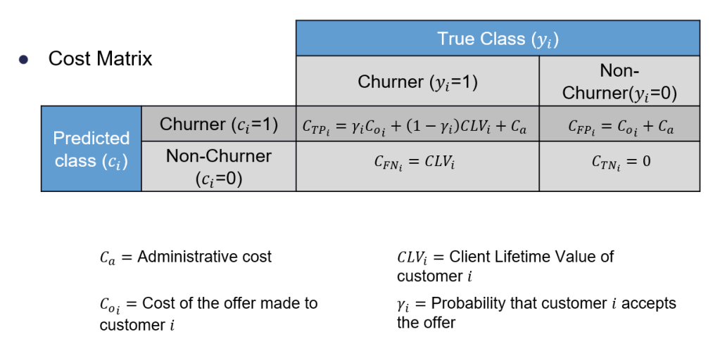
Using the Bayes minimum risk model with with the cost-sensitive matrix, defined in the part 1 of this posts:
We can now apply the model using the probabilities estimated with the three classification algorithms, decision tree, logistic regression and a random forest, used before. Let’s see the results measured by F1-Score and Savings

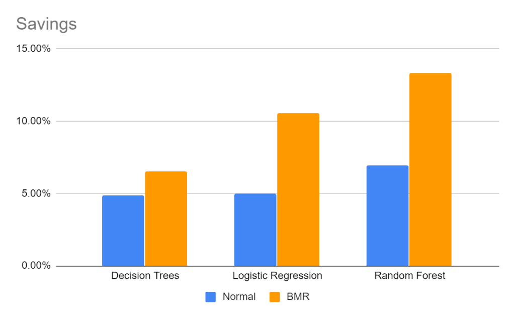
In blue we can see the results of each algorithm, as described in the previous post, then in orange we can observe the results of applying the Bayes Minimum Risk methodology.
The BMR algorithm generates an increase in savings and F1-Score regardless of the algorithm used. Nevertheless, the model with the highest savings is not the same as the one with the highest F1-Score.
In these three posts we have shown a new framework for a cost-sensitive churn machine learning. First, we show the importance of using the actual financial costs of the churn modeling process, since there are significant differences in the results when evaluating a churn campaign using a traditional such as the F1-Score, than when using a measure that incorporates the actual financial costs such as the savings. Moreover, we also show the importance of having a measure that differentiates the costs within customers, since different customers have quite a different financial impact as measured by their lifetime value.
Furthermore, our evaluations confirmed that including the costs of each example and using cost-sensitive methods lead to better results in the sense of higher savings. In particular, by using the cost-sensitive Bayes Minimum Risk algorithm, the financial savings are 13.36%, as compared to the savings of the cost-insensitive random forest algorithm which amount to just 6.94%.
