This post is part of a series in which I’m discussing several parts of my AI_at_Rappi presentation. In the latest post, we discussed how to evaluate a churn marketing campaign using a financial evaluation measure. In this one, we’re going to deep down in a couple of important concepts needed to fully being able to implement the aforementioned methodology. I’ll have to say that this post is going to be a bit more technical that the previous ones.
Financial evaluation of a churn model
In summary, assuming that every churner or that every prediction error have the same financial impact is not realistic. We showed how to estimate the savings of a given churn model using this cost matrix:
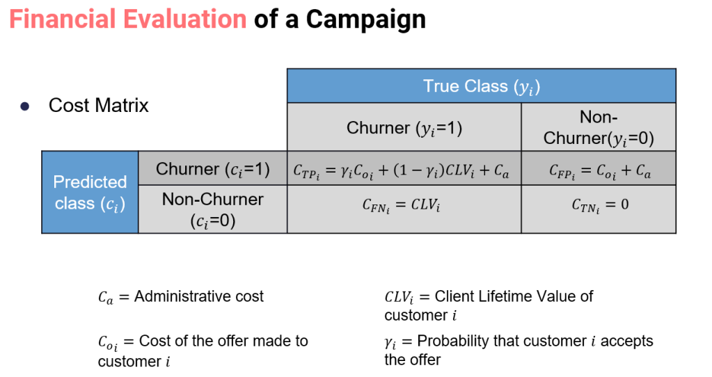
There are a couple terms that we missed to explain in the previous post, in particular the Customer Lifetime Value (CLV), the gamma probability, and also which offer to give to each customer.
Let’s first understand how to estimate the CLV.
Customer Lifetime Value

One of the key values to calculate the cost matrix, is the customer lifetime value. Within marketing there exists a common misconception between customer profitability and customer lifetime value. The two terms are usually used in an interchangeable way, creating confusion of what the actual objective of a churn modeling campaign should be. Several studies have proposed models providing a unique definition of both terms (Milne and Boza 1999; Neslin et al. 2006; Pfeifer et al. 2004; van Raaij et al. 2003). Customer profitability indicates the difference between the income and the cost generated by a customer i during a financial period t. It is defined as:

where 


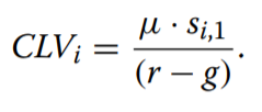
Moreover, we are interested to see what is the expected income that a particular customer will generate in the future, in other words, calculating the expected sum of discount future earnings (Neslin et al. 2006). Therefore, the 

where 


which in the case of 
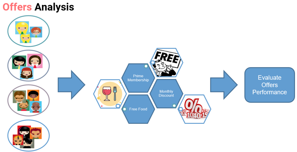
Offer Analysis
In practice companies have a set of offers to make to a customer as a part of the retention campaign, they vary from discounts, to upgrades among others. In the particular case of a marketplace such as Rappi, free deliveries, additional discounts, prime memberships and so on. Unsurprisingly, not all offers apply to all clients. For instance a customer that already has prime membership can not be offered that prime membership again. Moreover, an offer usually means an additional cost to the company and not all offers have not the same cost or the same impact in reducing churn.
Taking into account the cost and the implication of the offers, the problem can be resumed in making each customer the offer that will maximize the acceptance rate and more important reducing the overall cost.
In order to calculate the acceptance probability 

In this post we wanted to described with more details how to estimate the Customer Lifetime Value and also how it is possible to design experiments to estimate the probability of an offer acceptance gamma. Finally, in the next part of this cost-sensitive churn posts we’re planing to discuss how to include cost-sensitive machine learning algorithms into this analysis. Stay tuned.
